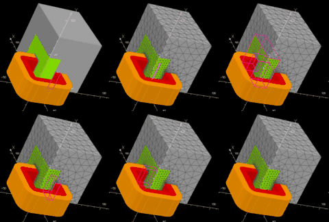
In the thermal modeling, the temperatures inside iron and core are from now on not uniform and it appears that the copper within magnetic circuit is hottest what conforms to physics.

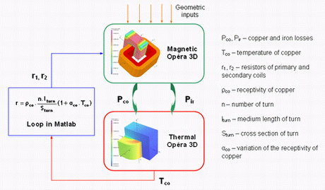
A magneto-thermal weak coupling is considered (Fig. 4). The copper and iron losses are computed with the magnetic AC solver and introduced as heat sources in the thermal static solver. The copper temperature is used to compute the coils resistors introduced in the magnetic solver and this loop continues until convergence of temperatures by using a fixed point algorithm. The Matlab script and Opera3D comi are given in the following file *.zip.

 

 

A. Analytical “coarse” model

The physical phenomena within the transformer are thermal, electric and magnetic. They are expressed in equations that are ranked using specific algorithms. The assumptions for the analytical models are uniform distribution of induction in the iron core and no voltage drop due to the magnetizing current. The magnetic field in coils is vertical.

This model leads to an implicit system of 8 equations and other equations solved sequentially. The non-linear implicit system is solved by using the Jacobean and the dogleg algorithm available in Matlab^® Optimization Toolbox. A complete description of the analytical model is available in the following files such as Matlab, MathCad, and Pro@Design.

B. 3D finite element “fine” model

Thermal and magnetic phenomena are both modeled by using 3D FEA. For the electromagnetic modeling, all magnetic and electric quantities are assumed sinusoidal. Full load and no-load simulations are used to compute all the characteristics. The iron loss is computed with Steinmetz formula and the leakage inductances are calculated with the magnetic co-energy.

 

 

 

 

 

 

 

 

 

 

 

 

Analytical & FEA models

Fig. 4. 3D FEA magneto-thermal weak coupling

Introduction | Optimization Problems | Models | Comparison | Combinatorial Opt. | Multi-Level Opt. |

Multi-Objective Opt. | Your results