Optimization methods
|
Date |
30/05/2007 |
|||||||||||||||||||||||||||||||||||||||||||||||
|
Author |
T.
V. Tran, S. Brisset, P. Brochet |
|||||||||||||||||||||||||||||||||||||||||||||||
|
Affiliation |
L2EP
– EC Lille – France |
|||||||||||||||||||||||||||||||||||||||||||||||
|
Email |
||||||||||||||||||||||||||||||||||||||||||||||||
|
Method |
Branch-and-bound |
|||||||||||||||||||||||||||||||||||||||||||||||
|
References |
[1] P. Venkataraman, Applied
Optimization with MatlabÒ Programming, A Wiley - Interscience publication, John
Wiley & Sons, New York, 2001. [2] Pro@Design, http://www.designprocessing.com |
|||||||||||||||||||||||||||||||||||||||||||||||
|
Description of the method |
A typical approach for handling discrete variables
is to solve the corresponding continuous optimization and then adjusts the
optimal design to neighboring discrete values [2].
But there is no guarantee that this process is correct or that a good
solution can be obtained by this way. One of efficient methods applied on the
combinatorial and mix engineering optimizations is Branch-and-Bound (BB)
method [1]. It is based on partial enumeration where only parts of the
combinations are explored. The BB algorithm uses a tree structure to
represent completions of partial solutions. The tree structure uses nodes and
edges to express the trail of partial solutions. The partial solution (one
node of the tree) is a solution in which some discrete variables are fixed
and others are free. It can be solved by a continuous optimization with
constraints applied. Thus the optimums of these partial solutions for a same
level are compared to find the minimum of them. This process continues
vertically as far as that all the variables are discrete and finally find the
minimal solution.
Fig.
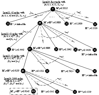
1. Branches and nodes of tree of the Branch-and-bound method. [ ] and { } denote respectively continuous and discrete variables Applied on this
Benchmark (fig. 1), the algorithm starts to break up “combinative branch”,
with four variables {a, b, c, d}. There are on the whole 62 branches.
Partial optimizations using Sequential Quadratic Programming algorithm (SQP)
with the variable remainder continuous S1, S2, n1
are launched with each branch combinative. The algorithm continues to
decompose last combinative branches with the variable S1, S2
and n1 compares with the previous optimum in order to
find the optimal solution. There are four
levels optimizations: the root node with all continuous variables; the first
nodes with 62 combinations of EIF and three continuous variables [S1,
S2, n1]; the second nodes with 63 combinations of S1
and two continuous variables [S2, n1]; the third
nodes with 63 combinations of S2 and one continuous
variable [n1]; and the fourth nodes with 1000 evaluations
of discrete variable n1. The partial solution of each node
with the objective function presented in the fig. 2 is really a successful
continuous optimization. This obtains a total mass Mnm
(|n is the number of branch; |m is
the level of tree). The minimal total mass of each optimization level is M*m.
This is taken and the other are cut out. Then the optimization levels
followed will be computed with these design discrete variables. Since this is a
combinatorial optimization problem with constraint non-linear applied, some
times the partial optimization can not be computed. In other words, no
constraints are active for all continuous optimization nodes. In this case, the algorithm returns to the
previous optimization level and takes the minimum following corresponding
with a new optimum design discrete variables. Then the combinative branch
continues decomposes. In the table I, the first minimal solution of level 1
is Table I Optimal Solutions Levels of
BB method
The level 4 is only 1000
evaluations with n1 and the minimal total mass with optimal
solution of discrete design variables is found M*tot.
|
|||||||||||||||||||||||||||||||||||||||||||||||
|
Publication of the method |
|
